import numpy as np
import pandas as pd
import time

import ipywidgets as widgets
from ipywidgets import interact, interactive

from bokeh.plotting import figure, show
from bokeh.io import output_notebook, push_notebook
from bokeh.models import LinearAxis, Range1d, ColumnDataSource
from bokeh.layouts import column, row

import numba

output_notebook()
# new code to detect whether running in google colab, and correctly setting working directory if so

#from os import path (not needed because os already loaded in cell above)

# mount google drive

# try command that only works when in google colab
try:

  from google.colab import drive
  in_colab = True
# if it fails, we are not running from google colab
except:
  in_colab = False
  print('Not in Colab')

# if we are in colab, mount the google drive and set working directory location to the standard download location
if in_colab:
  if os.path.exists('/content/google_drive'):
    print('Drive already mounted')
  else:
    drive.mount('/content/google_drive')

    # move working directory to file location
    #default should work, but change if using a different location
    %cd 'google_drive/MyDrive/Engineering_Hydrology_Notebooks/content/notebooks/Notebook_RR_Model'
    # Needs to be manually set for each notebook
Not in Colab
Conceptual Rainfall-Runoff Model#
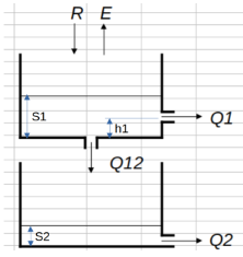
In this notebook, we’re going to set up and calibrate a basic conceptual rainfall-runoff model and calibrate it to some precipitation and runoff data. The conceptual model is as follows:
|
$\(Q_1 = a_1 \cdot (S_1 - h_{1})^{m_1}\)\( \)\(Q_{12} = a_{12} \cdot S_1^{m_{12}}\)\( \)\(Q_2 = a_{2} \cdot S_2^{m_2}\)$ |
 ]
]Import Climate Data#
We have observations of precipitation and runoff (and estimates of evaporation) at a frequency of 20 minutes. We would like to import them and set up empty vectors to represent the state variables for tank levels and the fluxes.
def initialize_df(df):
    # initialize the columns from the input data
    cols = ['S1 (mm)', 'Q1 (mm/h)', 'Q12 (mm/h)', 'S2 (mm)', 'Q2 (mm/h)', 'Q1+Q2 (mm/h)']
    df.loc[:, cols] = np.nan
    # calculate the timestep in minutes
    # df['Date'] = pd.to_datetime(df['Date'].to_numpy())
    # get the timestep and convert it to hours
    df['dt_hours'] = df['Date'].diff().dt.total_seconds().div(3600)
    # for some reason the Date column is unsorted, so sort it
    df.sort_values('Date', inplace=True)
    return df
raw_data = pd.read_csv('data/data.csv', parse_dates=['Date'], infer_datetime_format=True, dayfirst=True)
df = initialize_df(raw_data)
df.set_index('Date', inplace=True)
df.head()
| Rain (mm/h) | Evap (mm/h) | Runoff (mm/h) | S1 (mm) | Q1 (mm/h) | Q12 (mm/h) | S2 (mm) | Q2 (mm/h) | Q1+Q2 (mm/h) | dt_hours | |
|---|---|---|---|---|---|---|---|---|---|---|
| Date | ||||||||||
| 1987-09-02 00:20:00 | 0.0 | 0.0 | 0.038 | NaN | NaN | NaN | NaN | NaN | NaN | NaN |
| 1987-09-02 00:40:00 | 0.0 | 0.0 | 0.038 | NaN | NaN | NaN | NaN | NaN | NaN | 0.333333 |
| 1987-09-02 01:00:00 | 0.0 | 0.0 | 0.038 | NaN | NaN | NaN | NaN | NaN | NaN | 0.333333 |
| 1987-09-02 01:20:00 | 0.0 | 0.0 | 0.038 | NaN | NaN | NaN | NaN | NaN | NaN | 0.333333 |
| 1987-09-02 01:40:00 | 0.0 | 0.0 | 0.038 | NaN | NaN | NaN | NaN | NaN | NaN | 0.333333 |
# this will check if any value in any row is null (i.e. NaN)
# df[df[['Rain (mm/h)', 'Evap (mm/h)', 'Runoff (mm/h)']].isnull().any(axis=1)]
# plot_cols = [c for c in df.columns if c not in ['dt', 'Date']]

p_label = 'Rain (mm/h)'
q_label = 'Runoff (mm/h)'
e_label = 'Evap (mm/h)'
p = figure(title='Observed Precipitation and Runoff',
           x_axis_type='datetime', width=800, height=400)
p.line(df.index, df[q_label], line_width=2,
       legend_label=q_label, color='dodgerblue')
p.line(df.index, df[e_label], line_width=2,
       legend_label=e_label, color='orange')
p.xaxis.axis_label = 'Date'
p.yaxis.axis_label = q_label

p.extra_y_ranges = {"precip": Range1d(df[p_label].max(), 0)}
# data is in 20 minute intervals, and time is in milliseconds,
# so set width to 3.6E6 / 3
precip = p.vbar(
    x=df.index,
    top=0,
    bottom=df[p_label],
    width=20 * 60E3,
    y_range_name='precip',
    legend_label=p_label,
    alpha=0.5,
    color='lightseagreen',

)
precip.level = 'underlay'
p.add_layout(LinearAxis(axis_label=p_label, y_range_name='precip'), "right")

show(p)
def update_df():
    # if you are working in Jupyter lab, you can import the data just once.
    # However, there might be issues later on if you are updating the dataframe in
    # such a way that values from another iteration interfere.
    # it may be a case of just running a modified version of the 'initialize_df'
    # function where you just reset the desired columns to nan.  This won't take as much
    # time as reading the csv and converting the Date column to pandas datetime type.
    # df = initialize_df(pd.read_csv('data/data.csv', parse_dates=['Date'], dayfirst=True))
    # set_initial rain and evap as zero
    rain_0, evap_0 = 0, 0

    for i in range(0, len(df)):

        if i == 0:
            this_S1 = S1_init.value
            this_S2 = S2_init.value
        else:
            # get the timestep and convert it to hours
            dt = df.at[i, 'dt_hours']

            rain = df.at[i - 1, 'Rain (mm/h)']
            evap = df.at[i - 1, 'Evap (mm/h)']

            q1 = df.at[i - 1, 'Q1 (mm/h)']
            q12 = df.at[i - 1, 'Q12 (mm/h)']
            q2 = df.at[i - 1, 'Q2 (mm/h)']
            S1 = df.at[i - 1, 'S1 (mm)']
            S2 = df.at[i - 1, 'S2 (mm)']

            # since our dt is in hours and fluxes in mm/h
            # multiply by the timestep to get the sub-hourly fluxes
            delta_q1 = (rain - evap - q1 - q12) * dt
            # if i < 20:
            #     print(f'@dt={dt} delta q1 = {delta_q1:.3f}, rain={rain:.1f}, evap={evap:.1f}, q1={q1:.2f}, q12={q12:.2f}')
            this_s1 = max(0, S1 + delta_q1)

            delta_q2 = (q12 - q2) * dt
            this_s2 = max(0, S2 + delta_q2)

        # set reservoir levels for the current timestep
        df.at[i, 'S1 (mm)'] = this_S1
        df.at[i, 'S2 (mm)'] = this_S2

        # set flows for the current timestep based on current levels
        df.at[i, 'Q1 (mm/h)'] = a1.value * (this_S1 - h1.value)**m1.value
        df.at[i, 'Q12 (mm/h)'] = a12.value * (this_S1)**m12.value
        df.at[i, 'Q2 (mm/h)'] = a2.value * (this_S2)**m2.value
        df.at[i, 'Q1+Q2 (mm/h)'] = df.at[i, 'Q1 (mm/h)'] + df.at[i, 'Q2 (mm/h)']
    return df
Interactive Inputs#
@numba.jit(nopython=True)
def update_states_vectorized(rain, evap, dt, a1, m1, h1, a12, m12, a2, m2, S1_init, S2_init):
#     df = initialize_df(pd.read_csv('data/data.csv', parse_dates=True, infer_datetime_format=True))
    # for jit compiling, we need to initialize empty vectors
    # for each of the input columns from the pandas method
    s1, s2 = np.empty(len(rain)), np.empty(len(rain))
    q1, q2 = np.empty(len(rain)), np.empty(len(rain))
    q12 = np.empty(len(rain))
    q_tot = np.empty(len(rain))

    # set initial reservoir and outflow values
    s1[0] = S1_init
    s2[0] = S2_init
    q1[0] = 0 if s1[0] <= h1 else (a1 * (s1[0] - h1)**m1 ) * dt[1]
    q12[0] = (a12 * (s1[0])**m12) * dt[1]
    q2[0] = (a2 * s2[0]**m2) * dt[1]
    q_tot[0] = q1[0] + q2[0]

    for i in range(1, len(rain)):

        q1_balance = (rain[i-1] - evap[i-1] - q1[i-1] - q12[i-1]) * dt[i]
        this_S1 = max(0, s1[i - 1] + q1_balance)

        delta_q2 =  (q12[i - 1] - q2[i - 1]) / dt[i]
        this_S2 = max(0, s2[i - 1] + delta_q2)

        s1[i] = this_S1
        s2[i] = this_S2

        q1[i] = 0 if this_S1 <= h1 else (a1 * (this_S1 - h1)**m1) * dt[i]
        q12[i] = 0 if this_S1 <= 0 else (a12 * (this_S1)**m12) * dt[i]
        q2[i] = 0 if this_S2 <= 0 else (a2 * this_S2**m2) * dt[i]

        q_tot[i] = q1[i] + q2[i]

    return s1, s2, q1, q2, q12, q_tot
def vectorized_df_update(a1, m1, h1, a12, m12, a2, m2, S1_init, S2_init):
    p_label = 'Rain (mm/h)'
    e_label = 'Evap (mm/h)'
    rain = df[p_label].to_numpy()
    evap = df[e_label].to_numpy()
    dt = df['dt_hours'].to_numpy()
    s1, s2, q1, q2, q12, q_tot = update_states_vectorized(rain, evap, dt, a1, m1, h1, a12, m12, a2, m2, S1_init, S2_init)
    df['S1 (mm)'] = s1
    df['S2 (mm)'] = s2
    df['Q1 (mm/h)'] = q1
    df['Q2 (mm/h)'] = q2
    df['Q12 (mm/h)'] = q12
    df['Q1+Q2 (mm/h)'] = q_tot
    return df
def plot_model(a1, m1, h1, a12, m12, a2, m2, S1_init, S2_init):

    # df = update_df()
    df = vectorized_df_update(a1, m1, h1, a12, m12, a2, m2, S1_init, S2_init)
    source = ColumnDataSource(df)

    q_label = 'Runoff (mm/h)'
    sim_label = 'Q1+Q2 (mm/h)'

    fig = figure(width=800, height=300, x_axis_type='datetime',
                title='Observed vs. Simulated Runoff')

    # Plot Measured vs. Simuilated Runoff
    fig.line('Date', q_label, color='dodgerblue', line_width=2,
             legend_label='Observed', source=source)
    fig.line('Date', sim_label, color='navy', line_width=2,
             line_dash='dashed', legend_label='Simulated',
             source=source)

    fig.yaxis.axis_label = 'Runoff (mm/h)'

    # Tank 1 and Tank 2 flow plot
    f1 = figure(title='Tank 1 and 2 Flow', width=800, height=150,
               x_axis_type='datetime')
    f1.line('Date', 'Q1 (mm/h)', legend_label='Tank 1',
            line_width=2, color='purple', source=source)
    f1.line('Date', 'Q2 (mm/h)', legend_label='Tank 2',
            line_width=2, color='navy', source=source)
    f1.yaxis.axis_label = 'Runoff (mm/h)'

    # Regression Plot
    f2 = figure(width=400, height=450, title="Measured vs. Simulated Regression")
    f2.circle('Runoff (mm/h)', 'Q1+Q2 (mm/h)',
            source=source)


    # drop NaN values for Least-Squares fit
    df.dropna(inplace=True)

    # Best-fit line for regression plot
    fit = np.polyfit(df['Runoff (mm/h)'], df['Q1+Q2 (mm/h)'], 1)

    x = np.linspace(df['Runoff (mm/h)'].min(), df['Runoff (mm/h)'].max(), 100)
    y = [fit[0] * e + fit[1] for e in x]
    f2.line(x, y, color='red', line_dash='dashed')

    # calculate the R^2 and the NSE
    df['square_diff_Q1_Q2'] = (df['Runoff (mm/h)'] - df['Q1+Q2 (mm/h)'])**2

    # set a lower limit value to avoid divide by zero errors
    df = df[(df['Q1+Q2 (mm/h)'] != 0) & (df['Runoff (mm/h)'] != 0)].copy()
    df['log_square_diff_Q1_Q2'] = (np.log(df['Runoff (mm/h)']) - np.log(df['Q1+Q2 (mm/h)']))**2
    df['log_square_diff_Q1_Q2'] = df[np.isfinite(df['log_square_diff_Q1_Q2'])]['log_square_diff_Q1_Q2']
    nse = 1 - df['square_diff_Q1_Q2'].mean() / np.var(df['Runoff (mm/h)'])
#     log_nse = df['log_square_diff_Q1_Q2'].mean() / np.var(df['Runoff (mm/h)'])
    performance_str = f'Sim. vs. Obs Regression (NSE={nse:.2f})'
    f2.title = performance_str
    # print(performance_str)
    layout = row(column(fig, f1), f2)
    show(layout)
    # plt.annotate(performance_str, xy=(0, 0),
    #                xytext=(5, 340),
    #                textcoords="offset points",
    #                ha='left', va='center',
    #                color='black', weight='bold',
    #                clip_on=True)
from ipywidgets import TwoByTwoLayout, interactive_output, HBox
from IPython.display import display

a1 = widgets.FloatSlider(min=0., max=0.5, step=0.01, value=0.02, orientation='vertical', description='a1', continuous_update=False)
m1 = widgets.FloatSlider(min=0., max=2., step=0.01, value=1.0, orientation='vertical', description='m1', continuous_update=False)
h1 = widgets.FloatSlider(min=0., max=2., step=0.01, value=0.1, orientation='vertical', description='h1', continuous_update=False)
a12 = widgets.FloatSlider(min=0., max=0.5, step=0.01, value=0.021, orientation='vertical', description='a12', continuous_update=False)
m12 = widgets.FloatSlider(min=0., max=2., step=0.01, value=1., orientation='vertical', description='m12', continuous_update=False)
a2 = widgets.FloatSlider(min=0., max=1., step=0.01, value=0.2, orientation='vertical', description='a2', continuous_update=False)
m2 = widgets.FloatSlider(min=0., max=2., step=0.01, value=1.1, orientation='vertical', description='m2', continuous_update=False)
S1_init = widgets.FloatSlider(min=0., max=2., step=0.01, value=1.0, orientation='vertical', description='t1_init', continuous_update=False)
S2_init = widgets.FloatSlider(min=0., max=2., step=0.01, value=1.0, orientation='vertical', description='t2_init', continuous_update=False)

df = initialize_df(pd.read_csv('data/data.csv', parse_dates=['Date'], dayfirst=True))

sliders = {
    'a1': a1, 'm1': m1, 'h1': h1,
    'a12': a12, 'm12': m12,
    'a2': a2, 'm2': m2, 'S1_init': S1_init, 'S2_init': S2_init,
}
out = interactive_output(
    plot_model,
    sliders
)
display(HBox([a1, m1, h1, a12, m12, a2, m2, S1_init, S2_init]), out)
Examine Computational Performance#
Test the cycle time of the original function and compare to an updated (vectorized) function.
param_list = [('a1', 0.33),
              ('m1', 1.0),
              ('h1', 1.8),
              ('a12', 0.02),
              ('m12', 0.6),
              ('a2', 0.02),
              ('m2', 0.8),
              ('S1_init', 1.0),
              ('S2_init', 1.0)
             ]

params = {p[0]: max(0, np.random.normal(p[1])) for p in param_list}
# run some number of loops to generate an average execution time
times1, times2 = [], []
n_iterations = 10
for i in range(n_iterations):
    t0 = time.time()
    df = update_df()
    t1 = time.time()

    rain = df['Rain (mm/h)'].to_numpy()
    evap = df['Evap (mm/h)'].to_numpy()
    dt = df['dt_hours'].to_numpy()
    s1, s2, q1, q2, q12, q_tot = update_states_vectorized(rain=rain, evap=evap, dt=dt, **params)
    t2 = time.time()
    times1.append(t1 - t0)
    times2.append(t2 - t1)

mean1 = np.mean(times1)
mean2 = np.mean(times2)
print(f'Avg. of {n_iterations} iterations:')
print(f'    update_df: {mean1:.2f}/loop')
print(f'    update_df_update: {mean2:2f}/loop')
print(f'Vectorization speeds up computation ~{round(mean1/mean2, 0)}x')
Avg. of 10 iterations:
    update_df: 0.90/loop
    update_df_update: 0.027241/loop
Vectorization speeds up computation ~33.0x